Flow Machines with No Net Power Input¶

From the energy equation, we can also set the net power input to zero. In that case, the energy equation becomes:

(16)¶\[\left(h_e - h_0\right) + \frac{1}{2}\left(V_e^2 - V_0^2\right) = Q\]

Relating the kinetic energy term to the thrust via the conservation of momentum equation, we can write:

(17)¶\[\frac{1}{2}\left(V_e^2 - V_0^2\right) = \frac{1}{2}\left(V_e - V_0\right)\left(V_e + V_0\right) = V_{\text{avg}}\frac{F}{\dot{m}}\]

Plugging Eq. (17) into Eq. (16) and solving for the thrust, we find:

(18)¶\[F = \frac{\dot{m}}{V_{\text{avg}}} \left[Q - \left(h_e - h_0\right)\right]\]

For Eq. (18) to be positive, and therefore to be a thrust rather than a drag, the terms in square brackets must be larger than zero. This means that \(Q > 0\) (an input) and \(Q > (h_e - h_0)\). The heat transfer input typically comes from the combustion of a fuel with air in a jet engine.

Engine Designs¶

The specific choice of fuel and engine components depends on the operating speed range of the flow machine. In all air-breathing engine designs, an inlet, called a diffuser, captures air during flight. The air is mixed with fuel and ignited in the combustor, providing the input heat transfer. After combustion, the products are exhausted through a nozzle to produce thrust.

Note

In Section Assumptions, we assumed that the mass flow rate of the added fuel was negligible compared to the other flows in the engine. In principle, neglecting the fuel flow can cause between a 2-5% error in the mass flow rate. However, it happens that some air typically needs to be extracted for functions within the aircraft outside the engine. The mass flow rate of this bleed air, taken from the compressor, happens to be approximately equal to the mass flow rate of fuel added in the combustor. This reduces the error even further!

Turbojet¶

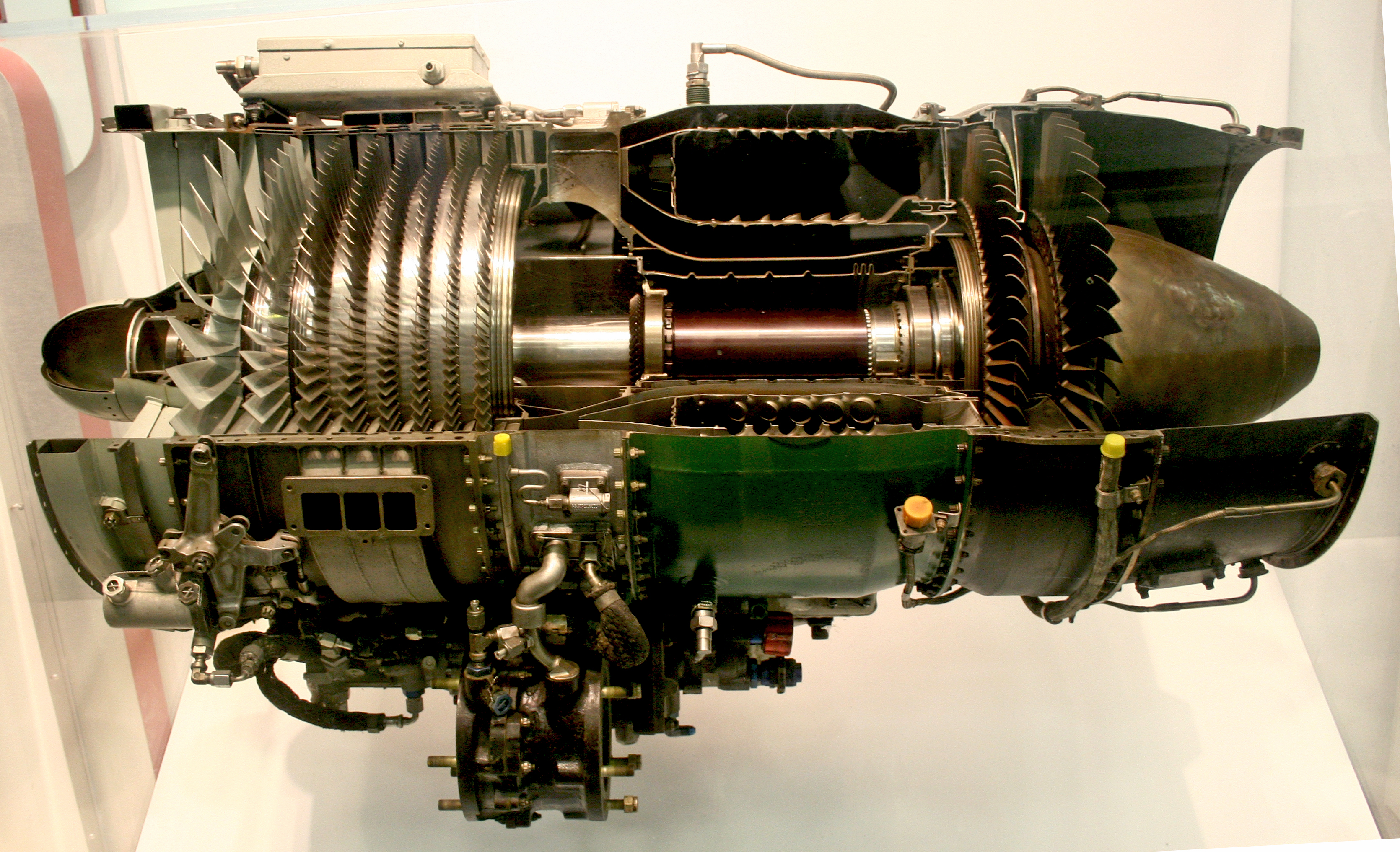
For flight Mach numbers in the range of 0 < \(M_0\) < 3, the pressure of the air must be increased after it is ingested. This is accomplished by a mechanical compressor, typically an axial compressor. To provide shaft power input to the compressor, a turbine is installed after the combustor, before the nozzle. The power extracted by the turbine exactly offsets the power input by the compressor, so the entire system has no net power. This engine design is called a turbojet engine, shown in Fig. 3 and Fig. 4, and the compressor and turbine are typically called turbomachinery.

Fig. 3 A schematic of a turbojet engine. Section numbers are indicated corresponding to states analyzed later.¶

../_images/J85_ge_17a_turbojet_engine.jpg

Fig. 4 A cut-away General Electric J85-GE-17A turbojet engine. Source: Wikimedia¶

One limitation of turbojet engines is that the amount of energy that can be added in the combustor is limited by the material properties of the downstream components. This is particularly true for the turbine, whose blades are rotating at extremely high RPM and are under very large stresses as a result. This temperature limit, in turn, limits the exhaust velocity \(V_e\), which limits the thrust output of a turbojet.

One way to cool the flow is by directing “cold” air from the compressor around the combustor and injecting it into the flow through cooling holes. Cooling holes are usually installed just downstream of the combustor and within the first few stages of turbine blades.

For steady state flight, we know that the thrust must equal the drag. However, in the transonic regime (0.8 < \(M_0\) < 1.2), the drag on the aircraft is significantly increased due to a phenomenon called drag-divergence. Drag divergence means that most turbojet powered aircraft cannot generate enough thrust to cruise at transsonic Mach numbers.

However, the engine can be modified to increase the amount of heat transfer input by adding an afterburner, as shown in Fig. 5. This is an additional combustor that is added between the turbine exit and the nozzle. Extra fuel is injected into the flow and ignited. Since there are no turbomachinery components downstream of the afterburner, the temperature can be much higher.

Fig. 5 A schematic of a turbojet engine including an afterburner.¶

Since cooling air is added to the flow to keep the turbine from failing, there is sufficient oxygen in the flow after the turbine to support more combustion. However, the total air-to-fuel ratio, which may be as high as 50 for standard turbojets, is halved to approximately 25 by the use of the afterburner. Due to this, afterburners are only included on aircraft intended for supersonic flight, mainly military aircraft.

Ramjet and Scramjet¶

At higher flight Mach numbers, between 3 < \(M_0\) < 5, a properly designed inlet can reduce the flow velocity to a subsonic velocity and compress the ingested air to high enough pressures that a compressor is not required. This pressure increase is called the ram pressure. Since no turbomachinery components are required, the design of the engine is substantially simplified. This design is called a ramjet, as shown in Fig. 6.

Fig. 6 A schematic of a ramjet or scramjet engine.¶

For flight Mach numbers greater than about 5, reducing the inlet flow to subsonic velocities would cause such a large temperature increase that any combustion would not be able to effectively provide heat transfer. Therefore, the inlet must be designed to reduce the flow velocity to a lower, but still supersonic, velocity. The inlet still provides a ram pressure increase, so no turbomachinery is required. This design is called a scramjet where the s and c stand for Supersonic Combustion ramjet.

Note

The biggest challenge with the design of scramjet engines is stabilizing the combustion within the engine. In a turbojet or ramjet engine, the flame is usually stabilized by introducing a flame holder, essentially a metal wedge, which causes the flow to recirculate. This mixes hot combustion products with fresh mixture, bringing the fresh mixture up to the ignition temperature. However, designers cannot use flame holders in scramjet engines because they would reduce the flow to subsonic velocity, with the accompaning temperature increase and pressure loss.

Eliminating turbomachinery simplifies the design of the ramjet and scramjet, but this comes with a major disadvantage. Ramjets and scramjets do not produce thrust unless they are flying at a high enough velocity to provide enough ram pressure. This means that they cannot accelerate from a standstill to their flight velocity. Instead, they must be started by launching from a high-speed platform, or have an additional on-board engine (for example, a rocket) to propel them to supersonic speeds.

Efficiency of Jet Engines¶

We can expand Eq. (18) with the definition of \(\dot{m}\) and \(V_{\text{avg}}\) to find:

(19)¶\[F = \rho_0 A_0 \frac{V_0}{\left(V_0 + V_e\right)/2} \left[Q - \left(h_e - h_0\right)\right]\]

As flight velocity \(V_0\) increases, both the top and bottom of the fraction in the middle of Eq. (19) will increase. This means that the thrust is approximately constant as flight speed changes. This is the primary advantage of jet engines over propellers, because it is not inherently speed-limited.

Overall Efficiency¶

To define the overall efficiency of the propulsion engine, we can take the ratio of the useful power output to the rate of heat transfer input:

(20)¶\[\eta_o = \frac{F V_0}{\dot{m}Q} = \frac{V_0}{V_{\text{avg}}} \left[1 - \frac{h_e - h_0}{Q}\right]\]

In Eq. (20), we identify the ratio \(V_0/V_{\text{avg}}\) as the propulsive efficiency, \(\eta_{\text{p}}\). In addition, we can define the thermal efficiency as:

(21)¶\[\eta_{\text{th}} = 1 - \frac{h_e - h_0}{Q}\]

This means we can represent the overall thermal efficiency as:

\[\eta_o = \eta_{\text{p}} \eta_{\text{th}}\]

The thermal efficiency captures the imperfect conversion of heat input to usable thermal energy, since some energy is stored in the flow of gases. The propulsive efficiency captures the effect of imperfect conversion of thrust into velocity change.

In a typical jet engine, these two efficiencies move in opposite directions. When the thermal efficiency is high, the exit velocity is high as well. This leads to a lower propulsive efficiency for a given flight speed. Typical jet aircraft will cruise around \(V_0/V_e \approx 0.6\), which represents a good balance between the two efficiencies.

Fuel Efficiency¶

A separate metric from the overall efficiency of the engine is the fuel efficiency. Whereas the overall efficiency is related to the thermodynamic state of the engine, the fuel efficiency is explicitly related to the consumption of fuel.

For engines that rely on heat input, the heat added to the flow, \(\dot{m}Q\), is proportional to the flow rate of fuel, \(\dot{m}_{\text{f}}\) and the heat of combustion of the fuel, \(Q_{\text{f}}\). The constant of proportionality is called the burner efficiency, \(\eta_{\text{b}}\):

(22)¶\[\dot{m} Q = \eta_{\text{b}} \dot{m}_{\text{f}} Q_{\text{f}}\]

The heat of combustion of the fuel, also called the heating value of the fuel, is a property of the fuel. Well-designed combustors in jet engines can achieve values of \(\eta_{\text{b}}\) in excess of 90%. This implies that more than 90% of the chemical energy of the fuel is transferred into the flow, and the rest is transferred to the structure of the combustor or engine.

The most common metric for fuel consumption in jet engines is thrust-specific fuel consumption, TSFC, given the symbol \(c_{\text{j}}\). TSFC is defined as the mass flow rate of fuel, usually in mass per hour, divided by the thrust force:

\[c_{\text{j}} = \frac{\dot{m}_{\text{f}}}{F}\]

The reason why TSFC is preferred over just the fuel flow rate is for the same reason that miles-per-gallon are preferred for automobiles. That is, it is known that generating more thrust (going more miles) will take more mass of fuel (more gallons of fuel), so it is not very interesting that it takes more fuel. What’s more important is how efficient you are at generating that thrust or going that number of miles.

We can combine the equations for the overall efficiency, Eq. (20), and the burner efficiency, Eq. (22), to simplify the TSFC:

(23)¶\[c_{\text{j}} = \frac{V_0}{\eta_{\text{o}}\eta_{\text{b}}Q_{\text{f}}} = \frac{V_0}{\eta_{\text{p}}\eta_{\text{th}}\eta_{\text{b}}Q_{\text{f}}} = \frac{V_{\text{avg}}}{\eta_{\text{th}}\eta_{\text{b}}Q_{\text{f}}}\]

This equation shows us that higher thermal efficiency, burner efficiency, propulsive efficiency, or higher heat of combustion all result in a smaller TSFC. On the other hand, higher flight velocity or higher exhaust velocity result in larger TSFC. A simplified analysis shows us that the TSFC is approximately a linear function of the flight Mach number, \(M_0\).

Example¶

Assume that a JTC3 engine is operating at sea level on a test stand, burning Jet-A fuel with a burner efficiency of 96%. The engine is producing 50 kN of thrust while ingesting 81.5 kg/s of air. The engine is operating at full power and the temperature in the pressure-equilibrated exhaust is measured to be \(T_e\) = 655 K. What is the TSFC of this engine under these conditions? Assume that \(T_0\) = 288 K.

We can combine Eq. (18) with Eq. (22) to find:

\[F = \frac{\dot{m}_{\text{f}}}{V_{\text{avg}}}\eta_{\text{b}}Q_{\text{f}} - \frac{\dot{m}}{V_{\text{avg}}}\left(h_e - h_0\right)\]

Rearranging to solve for \(c_{\text{j}} = \dot{m}_{\text{f}}/F\), we find:

\[c_{\text{j}} = \frac{\dot{m}_{\text{f}}}{F} = \frac{V_{\text{avg}}}{\eta_{\text{b}}Q_{\text{f}}-\dot{m}/\dot{m}_{\text{f}}\left(h_e - h_0\right)}\]

Note that there are three unknowns in this equation, \(V_e\), \(\dot{m}_{\text{f}}\), and the ratio \(\dot{m}/\dot{m}_{\text{f}}\). Next, we turn to the momentum conservation equation. Although we previously assumed that additional mass flows could be neglected, we need some way to determine the mass flow rate ratio, so we modify the momentum conservation equation to include the fuel mass flow rate:

\[F = \left(\dot{m}_0 + \dot{m}_{\text{f}}\right)V_e - \dot{m}_0 V_0\]

where \(\dot{m}_0=\dot{m}\) is the ingested air mass flow rate. Solving this equation for \(c_{\text{j}}\), we find:

\[c_{\text{j}} = \frac{\dot{m}_{\text{f}}}{F} = \frac{\dot{m}_{\text{f}}/\dot{m}_0}{\left(1 + \dot{m}_{\text{f}}/\dot{m}_0\right)V_e - V_0}\]

The final equation we need is to rearrange the thrust equation and solve for \(V_e\). We note that since the engine is on a test stand, the inlet velocity is zero, \(V_0 = 0\):

\[V_e = \frac{F}{\dot{m}_0 \left(1 + \dot{m}_{\text{f}}/\dot{m}_0\right)}\]

We now have three equations and three unknowns:

\(V_e\)
\(c_{\text{j}}\)
\(\dot{m}_{\text{f}}/\dot{m}_0\)

We can solve these algebraically, but in this case I think it’s easier to guess a value for \(\dot{m}_{\text{f}}/\dot{m}_0\) and solve iteratively. We will guess a value of \(\dot{m}_{\text{f}}/\dot{m}_0\) = 0.02.

from pint import UnitRegistry
units = UnitRegistry()

mdot_0 = 81.5 * units.kg / units.s
F = 50 * units.kN
T_0 = 288 * units.K
T_e = 655 * units.K
eta_b = 0.96 * units.dimensionless
Q_f = 43.4 * units.MJ / units.kg

# From table B-2
c_pe = 1.11 * units.kJ / (units.kg * units.K)
c_p0 = 1.03 * units.kJ / (units.kg * units.K)
delta_h = c_pe * T_e - c_p0 * T_0

f_a_guess = 0.02 * units.dimensionless

V_e_guess = (F / (mdot_0 * (1 + f_a_guess))).to("m/s")
print(f"{V_e_guess=}")

c_j_1 = (f_a_guess / ((1 + f_a_guess) * V_e_guess)).to("kg/hr/N")
c_j_2 = (0.5 * V_e_guess / (eta_b * Q_f - 1 / f_a_guess * delta_h)).to("kg/hr/N")
print(f"{c_j_1=}", f"{c_j_2=}", sep="\n")

V_e_guess=<Quantity(601.467581, 'meter / second')>
c_j_1=<Quantity(0.11736, 'kilogram / hour / newton')>
c_j_2=<Quantity(0.0537464515, 'kilogram / hour / newton')>

Those two values for \(c_{\text{j}}\) don’t match, and c_j_1 is larger than c_j_2. Since f_a_guess is in the numerator of c_j_1, which we need to make smaller, we’ll guess a smaller value for f_a_guess. Let’s guess \(\dot{m}_{\text{f}}/\dot{m}_0\) = 0.01.

f_a_guess = 0.01 * units.dimensionless

V_e_guess = (F / (mdot_0 * (1 + f_a_guess))).to("m/s")
print(f"{V_e_guess=}")

c_j_1 = (f_a_guess / ((1 + f_a_guess) * V_e_guess)).to("kg/hr/N")
c_j_2 = (0.5 * V_e_guess / (eta_b * Q_f - 1 / f_a_guess * delta_h)).to("kg/hr/N")
print(f"{c_j_1=}", f"{c_j_2=}", sep="\n")

V_e_guess=<Quantity(607.422705, 'meter / second')>
c_j_1=<Quantity(0.05868, 'kilogram / hour / newton')>
c_j_2=<Quantity(-0.794016608, 'kilogram / hour / newton')>

Still no match, but we made c_j_1 smaller, which is good. Unfortunately, the sign of c_j_2 is negative, so we went too far. The answer is between 0.02 and 0.01. Let’s try 0.015.

f_a_guess = 0.015 * units.dimensionless

V_e_guess = (F / (mdot_0 * (1 + f_a_guess))).to("m/s")
print(f"{V_e_guess=}")

c_j_1 = (f_a_guess / ((1 + f_a_guess) * V_e_guess)).to("kg/hr/N")
c_j_2 = (0.5 * V_e_guess / (eta_b * Q_f - 1 / f_a_guess * delta_h)).to("kg/hr/N")
print(f"{c_j_1=}", f"{c_j_2=}", sep="\n")

V_e_guess=<Quantity(604.430475, 'meter / second')>
c_j_1=<Quantity(0.08802, 'kilogram / hour / newton')>
c_j_2=<Quantity(0.0838839519, 'kilogram / hour / newton')>

Based on our previous results, since c_j_1 > c_j_2, the actual fuel/air ratio is smaller than the guess value. Let’s try 0.0125.

f_a_guess = 0.0125 * units.dimensionless

V_e_guess = (F / (mdot_0 * (1 + f_a_guess))).to("m/s")
print(f"{V_e_guess=}")

c_j_1 = (f_a_guess / ((1 + f_a_guess) * V_e_guess)).to("kg/hr/N")
c_j_2 = (0.5 * V_e_guess / (eta_b * Q_f - 1 / f_a_guess * delta_h)).to("kg/hr/N")
print(f"{c_j_1=}", f"{c_j_2=}", sep="\n")

V_e_guess=<Quantity(605.922896, 'meter / second')>
c_j_1=<Quantity(0.07335, 'kilogram / hour / newton')>
c_j_2=<Quantity(0.15082714, 'kilogram / hour / newton')>

Too far again, so the answer is between 0.0125 and 0.015. Let’s try the midpoint again, 0.01375.

f_a_guess = 0.01375 * units.dimensionless

V_e_guess = (F / (mdot_0 * (1 + f_a_guess))).to("m/s")
print(f"{V_e_guess=}")

c_j_1 = (f_a_guess / ((1 + f_a_guess) * V_e_guess)).to("kg/hr/N")
c_j_2 = (0.5 * V_e_guess / (eta_b * Q_f - 1 / f_a_guess * delta_h)).to("kg/hr/N")
print(f"{c_j_1=}", f"{c_j_2=}", sep="\n")

V_e_guess=<Quantity(605.175766, 'meter / second')>
c_j_1=<Quantity(0.080685, 'kilogram / hour / newton')>
c_j_2=<Quantity(0.105131608, 'kilogram / hour / newton')>

Not far enough, the true answer is between 0.01375 and 0.015. The midpoint is now 0.014375.

f_a_guess = 0.014375 * units.dimensionless

V_e_guess = (F / (mdot_0 * (1 + f_a_guess))).to("m/s")
print(f"{V_e_guess=}")

c_j_1 = (f_a_guess / ((1 + f_a_guess) * V_e_guess)).to("kg/hr/N")
c_j_2 = (0.5 * V_e_guess / (eta_b * Q_f - 1 / f_a_guess * delta_h)).to("kg/hr/N")
print(f"{c_j_1=}", f"{c_j_2=}", sep="\n")

V_e_guess=<Quantity(604.802891, 'meter / second')>
c_j_1=<Quantity(0.0843525, 'kilogram / hour / newton')>
c_j_2=<Quantity(0.092868523, 'kilogram / hour / newton')>

We can now continue this process until we find an answer that meets our desired accuracy criteria. This is called the bisection method because we are bisecting the search space with each iteration. Continuing until we have 4 digits of agreement in the TSFC:

f_a_guess = 0.0147815 * units.dimensionless

V_e_guess = (F / (mdot_0 * (1 + f_a_guess))).to("m/s")
print(f"{V_e_guess=}")

c_j_1 = (f_a_guess / ((1 + f_a_guess) * V_e_guess)).to("kg/hr/N")
c_j_2 = (0.5 * V_e_guess / (eta_b * Q_f - 1 / f_a_guess * delta_h)).to("kg/hr/N")
print(f"{c_j_1=}", f"{c_j_2=}", f"{c_j_2.to('lb/hr/lbf')=}", sep="\n")

V_e_guess=<Quantity(604.56062, 'meter / second')>
c_j_1=<Quantity(0.086737842, 'kilogram / hour / newton')>
c_j_2=<Quantity(0.0867386029, 'kilogram / hour / newton')>
c_j_2.to('lb/hr/lbf')=<Quantity(0.85061512, 'pound / force_pound / hour')>

We find that the value here is about 8% higher than the quoted value for the TSFC on Wikipedia.

Notes for Propulsion